Projected Conjugate Gradient
The projected conjugate gradient (CG) method was implemented during my first GSoC weeks. It solves the equality-constrained quadratic programming (EQP) problems of the form:
\begin{eqnarray}
\min_x && \frac{1}{2} x^T H x + c^T x + f, \\
\text{subject to } && A x = b.
\end{eqnarray}
This method is used by a variety of algorithms for linearly and nonlinearly constrained optimization and is an important substep of the nonlinear programming solver I am implementing and, therefore, deserve some discussion. I based my implementation on the descriptions in [1], Chapter 16, and in [2].
Conjugate Gradient
Before explaining the projected conjugate gradient, a brief explanation about the conjugate gradient method will be provided. The conjugate gradient (CG), is a procedure to solve the problem:
\begin{equation} \min_x ~ \phi(x) = \frac{1}{2} x^T H x + c^T x+f, \end{equation}
for a symmetric positive definite matrix $H$. Which happens to be equivalent to the problem of finding a solution to the problem $H x = -c$.
The CG method is an iterative procedure, that starts with a initial solution $x_0$ and update this solution iteratively:
\begin{equation} x_{k+1} = x_{k} + \alpha_k p_k. \end{equation}
The name of the method is due to a property of the update vectors $p_k$: these vectors are said to be conjugate with respect to $H$ because they satisfy the following property:
\begin{equation} p_i^T H p_j = 0,~\text{for all }i \not= j. \end{equation}
It is easy to prove the conjugacy of the a set of vectors $\{p_0,\cdots, p_k\}$ is sufficient to guarantee this set is linearly independent.
After $n$ iteration the resulting vector is:
\begin{equation} x_n = x_0 + \alpha_0 p_0 + \cdots + \alpha_{n-1} p_{n-1}, \end{equation}
since we have the sum of $n$ linear independent vectors. If $x_n\in \mathbb{R}^n$ for the right choice of coefficients $\alpha_k$ we have that $x_n$ can assume any value in $\mathbb{R}^n$, inclusive the optimal value $x^*$ that is solution to the problem of minimizing $\phi(x)$. And, therefore, the CG method converge in at most $n$ iterations.
The strength of the conjugate gradient method is that a satisfactory solution to the minimization problem can usually be obtained in much less than $n$ iterations. Furthermore, the set of conjugate vectors $\{p_0,\cdots, p_k\}$ is computed in rather economic fashion by using only the previous value $p_{k}$ to compute the new conjugate vector $p_{k+1}$:
\begin{equation} p_{k+1} = r_{k+1} + \beta_k p_{k}, \end{equation}
where $r_k$ is the gradient of $\phi$ evaluated in $x_k$:
\begin{equation} r_{k} = \nabla \phi(x_k) = H x_k + c, \end{equation}
and $\beta_k$ is constant chosen such that if $p_{k}$ is conjugate to the set $\{p_0,\cdots, p_k-1\}$ than $p_{k+1}$ is conjugate to this set too and also to $p_{k}$.
The constant $\alpha_k$ and $\beta_k$ can be easily compute using the following formulas:
\begin{eqnarray}
\alpha_k = \frac{r_k^T r_k}{p_k H p_k} \\
\beta_k = \frac{r_{k+1}^T r_{k+1}}{r_k^T r_k}.
\end{eqnarray}
For a explanation on how this constants were compute we refer the reader to [1], Chapter 5 .
Now we are ready to present the basic operations performed in a single iteration of the CG method:
- Compute $\alpha_k = \frac{r_k^T r_k}{p_k H p_k}$;
- Update the solution $x_{k+1} = x_{k} + \alpha_k p_k$;
- Compute the residual $r_{k+1} = H x_{k+1} + c$;
- Compute $\beta_k = \frac{r_{k+1}^T r_{k+1}}{r_k^T r_k}$;
- Get a new conjugate vector: $p_{k+1} = r_{k+1} + \beta_k p_{k}$
This method can be implement in quite economic fashion without the need to actually store the matrix $H$. Only the ability to compute the product $H v$ for any given vector $v$ is actually need, which makes this method very appropriate for very large problems.
A comprehensive description of the CG method can be found in [1], Chapter 5.
Projected Conjugate Gradient
The projected CG method is a variation of the CG method that is able to solve Equality-constrained Quadratic Programming (EQP) problems of the form:
\begin{eqnarray}
\min_x && \phi(x) = \frac{1}{2} x^T H x + c^T x + f, \\
\text{subject to } && A x = b.
\end{eqnarray}
The idea of this method is to choose an initial point $x_0$, such that $x_0$ satisfy the constraints:
\begin{equation} A x_0 = b, \end{equation}
and to choose the update vectors $p_k$ in the null space of $A$:
\begin{equation} A p_k = 0, \end{equation}
It follows that for:
\begin{equation} x_k = x_0 + (\alpha_0 p_0 + \cdots + \alpha_{n-1} p_{k-1}), \end{equation}
we have $A x_k = A x_0 + 0 = b$. Such that the constraints are satisfied along the iterations, while $x_k$ get progressively close to the actual solution of the EQP problem.
A comprehensive description of the projected CG method can be found on [1], Chapter 16.
Roundoff Errors
A naive implementation of the projected CG method may have it result significantly affected by roundoff errors.
The problem occurs because the computed vector $p_k$ may not be exactly on the null-space of the matrix $A$, such that:
\begin{equation} A p_k > 0, \end{equation}
This cause the constraints to be progressively more violated along the iterations.
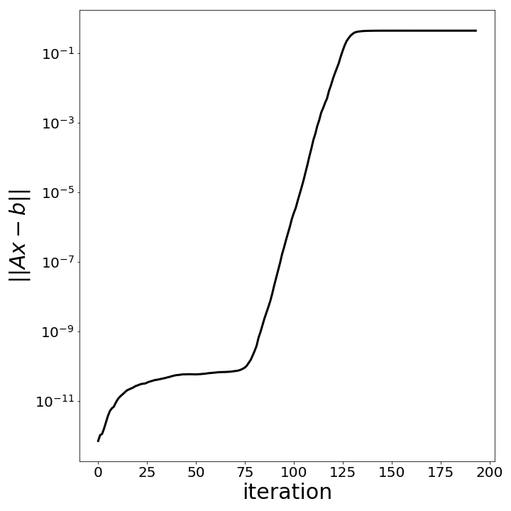
The next figure shows the application of the projected CG
for the problem CVXQP3_M from the CUTEst collection.
The constrain violation $\|Ax_k-b\|$ is monitored
along the iterations, showing that the roundoff errors
can results in very large constraints violations.
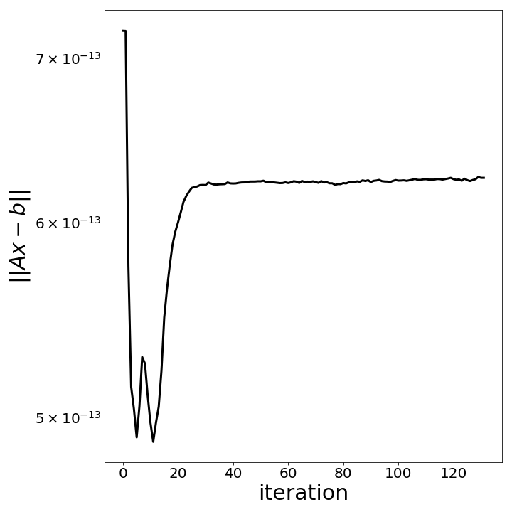
Fortunately, in [2] some iterative refinements and a new way to update the residuals are proposed to keep the roundoff errors at acceptable levels. The constrain violation $\|Ax_k-b\|$ along the iterations, after implementing the proposed modifications, is displayed bellow (indicating acceptable levels of constraint violation along the iterations).
Final Results
I performed experiments on the following set of problems:
CVXQP1_S, CVXQP2_S, CVXQP3_S, CVXQP1_M, CVXQP2_M, CVXQP3_M,
CVXQP1_L, CVXQP2_L, CVXQP3_L, CONT-050, CONT-100, DPKL01, MOSARQP1,
DUAL1, DUAL2, DUAL3, DUAL4, PRIMAL1, PRIMAL2, LASER
from
the CUTEst colection.
The description of the problems can be found in [3] (convex QP problems).
I compared two variations of the projected CG method (both of them using the refinements described in [2]) with the solution of the EQP problem by the direct factorization of the Karush-Kuhn-Tucker equations. The two variations are refered as normal equation approach and augmented system approach (as they are named in [2]).
The comparison is presented on the graph below, each problem solution being represented by a dot on an “optimality measure $\phi(x)$ vs the constraint violation $\|Ax_k-b\|$” plane. Each problem was solved by the three different methods and solutions obtained throght different methods are being represented by different colors.
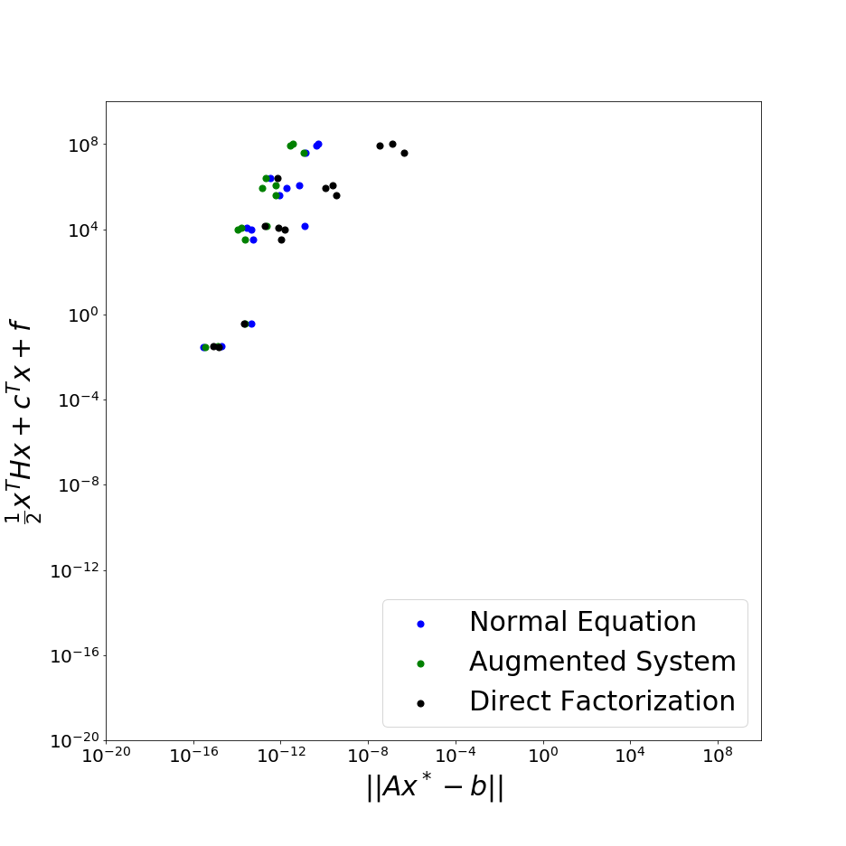
The augmented system approach seems to provide a slightly more accurate result compared with the normal equation approach. And both projected CG methods seems very competitive with the direct factorization approach, in terms of accuracy.
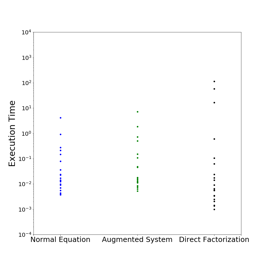
About the execution time: The normal equation approach is slightly (no more than 2x) faster than the augmented system approach. The direct factorization is significantly slower (more than 10x) for very large problems and can be slightly faster for small problems compared to both CG methods. The executions times (in seconds) are compared on the graph bellow for the same set of problems.
References
[1] Jorge Nocedal, and Stephen J. Wright. “Numerical optimization” Second Edition (2006).